Usage

Here we assume you use a HDF5 database. The FITS format will be discontinued soon.

Listing synthesis runs

Start a python shell. To list the synthesis runs present in the database qalifa-synthesis.h5, use the function listRuns():

>>> from pycasso.h5datacube import *
>>> listRuns('qalifa-synthesis.h5')
eBR_v20_q027.d13c512.ps3b.k1.mC.CCM.Bgsd01.v01
eBR_v20_q036.d13c512.ps03.k2.mC.CCM.Bgsd61

In this case, we have two runs, 'eBR_v20_q027.d13c512.ps3b.k1.mC.CCM.Bgsd01.v01' and 'eBR_v20_q036.d13c512.ps03.k2.mC.CCM.Bgsd61'. The other tools for listing the contents of a database are listBases() and listQbickRuns().

>>> listBases('qalifa-synthesis.h5')
Bgsd01
Bgsd61
>>> listQbickRuns('qalifa-synthesis.h5')
q027
q036

Now, we can search the runs that have specific bases or qbick runs using the keyword arguments baseId and qbickRunId. One can specify any one or both of these filter arguments.

>>> listRuns('qalifa-synthesis.h5', baseId='q036', qbickRunId='Bgsd61')
eBR_v20_q036.d13c512.ps03.k2.mC.CCM.Bgsd61

Loading galaxy data

To load the galaxy 'K0001', in the run 'eBR_v20_q036.d13c512.ps03.k2.mC.CCM.Bgsd61' from the database, do

>>> from pycasso.h5datacube import *
>>> K = h5Q3DataCube('qalifa-synthesis.h5', 'eBR_v20_q036.d13c512.ps03.k2.mC.CCM.Bgsd61', 'K0001')

The object K is a h5Q3DataCube. If you are using ipython, entering K followed by two tab keystrokes, you should see all the properties of the galaxy and all methods available to operate on those.

Zone smoothing

The data from the galaxies are are binned in spatial regions called voronoi bins. There is a procedure called “dezonification” which converts the data from voronoi bins back to spatial coordinates. When doing so, one can use the surface brightness of the image of the galaxy as a hint to smooth some of the properties.

This is enabled by default. To disable it, set the keyword argument smooth to False when loading the galaxy.

>>> K = h5Q3DataCube('qalifa-synthesis.h5', 'eBR_v20_q036.d13c512.ps03.k2.mC.CCM.Bgsd61', 'K0001', smooth=False)

For more information, see getDezonificationWeight().

Displaying property images

In this section we explain how to obtain images of properties of the galaxy. Most of of the properties of interest are already calculated, see the section Galaxy property list.

Here we assume the galaxy is loaded as K. Now, all the data is stored as voronoi zones, but we really want to see the spatial distribution of the galaxy properties. K has a method for converting data from voronoi zones to images, the method zoneToYX().

Let’s see the property popx. It is a 3-dimensional array, containing the light fraction for every triplet (age, metallicity, zone).

>>> K.popx.shape
(39, 4, 649)
>>> K.N_age, K.N_met, K.N_zone
(39, 4, 649)

Now, we want to see how this is distributed in the galaxy. The fraction of light in each population is the same in every pixel of a zone. So, we call popx an intensive property. To inform zoneToYX() that the property is intensive, we set extensive=False.

>>> popx = K.zoneToYX(K.popx, extensive=False)
>>> popx.shape
(39, 4, 72, 77)

Now, the resulting popx is 4-dimensional, where the zone dimension has been replaced by the (x,y) plane. Let’s plot the young population (summing only the fractions for ages smaller than 1Gyr) as a function of the position in the galaxy plane.

>>> import matplotlib.pyplot as plt
>>> popY = popx[K.ageBase < 1e9].sum(axis=1).sum(axis=0)
>>> plt.imshow(popY, origin='lower', interpolation='nearest')
>>> cb = plt.colorbar()
>>> cb.set_label('[%]')
>>> plt.title('light fraction < 1 Gyr')

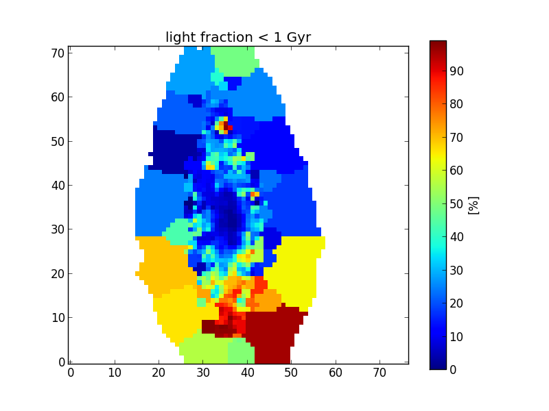
Masked pixels

The white pixels do not belong to any zone (masked pixels), and by default are set to numpy.nan. One might change the fill value for the masked pixels using the keyword fill_value. For example, to fill with zeros,

>>> popx_fill_zeros = K.zoneToYX(K.popx, extensive=False, fill_value=0.0)

It is recommended to use the fill values as nan, this way you know when you make a mistake and use value for regions where there’s no data (nan is contagious, any operation containing a nan will result nan).

Surface densities

When the property is extensive, such as mass or flux, it is more proper to work with surface densities of these properties, when working with images. The most easily acknowledged extensive properties are light and mass. The properties Lobn__z, Mini__z and Mcor__z are the total light and mass for the voronoi zones. When we convert these to images, setting extensive=True, the resulting image contains the surface density of these properties (for example, in units of \(M_\odot / pc^2\)).

>>> McorSD = K.zoneToYX(K.Mcor__z, extensive=True)
>>> plt.imshow(McorSD, origin='lower', interpolation='nearest')
>>> cb = plt.colorbar()
>>> cb.set_label('$[M_\odot / pc^2]$')
>>> plt.title('McorSD')

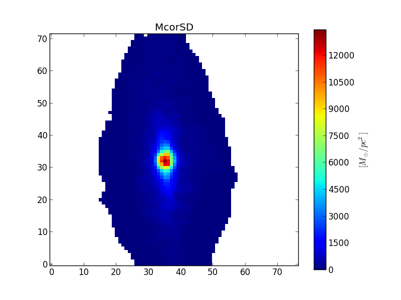
This is the same property as McorSD__yx.

Radial and azimuthal profiles

Galaxy images are nice and all, but in the end you want to compare spatial information between galaxies, and it can not be done in a per pixel basis. One can think in polar coordinates and analyze only the radial variations of the properties. For this we have to think about what galaxy distances in these images really mean.

Image geometry

One fair approximation is to assume the galaxy has an axis-symmetric geometry. Therefore, if we see the galaxy as an elliptic shape, that is because of its inclination with respect to the line of sight. If we get all the points at a given distance a from the center of the galaxy, this will appear as an ellipse of semimajor axis equal to a.

To know the distace of each pixel to the center of the galaxy, we need to know the ellipticity (ba) of the galaxy, defined as \(\frac{b}{a}\) (ratio between semiminor and semimajor axes), and the position angle (pa, in radians, counter-clockwise from the X-axis) of the ellipse. These can be set using the method setGeometry(). The distance of each pixel is obtained using the property pixelDistance__yx.

>>> K.setGeometry(pa=45*np.pi/180.0, ba=0.75)
>>> dist = K.pixelDistance__yx
>>> plt.imshow(dist, origin='lower', interpolation='nearest')
>>> cb = plt.colorbar()
>>> cb.set_label('pixels')
>>> plt.title('Pixel distance')

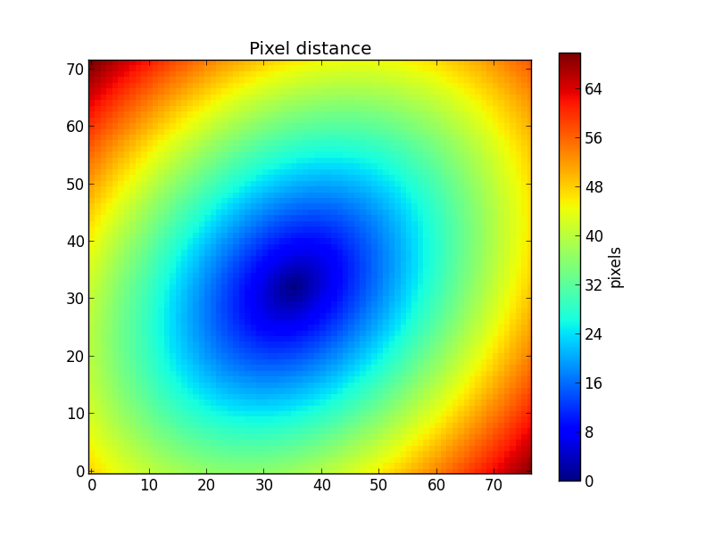
This example geometry clearly does not correspond to geometry of the galaxy, as seen in the previous figures. If we lack the values of ba and pa from other sources, we can use the method getEllipseParams() to estimate these ellipse parameters using “Stokes’ moments” of the flux (actually, we use qSignal) as explained in the paper Sloan Digital Sky Survey: Early Data Release.

>>> pa, ba = K.getEllipseParams()
>>> K.setGeometry(pa, ba)

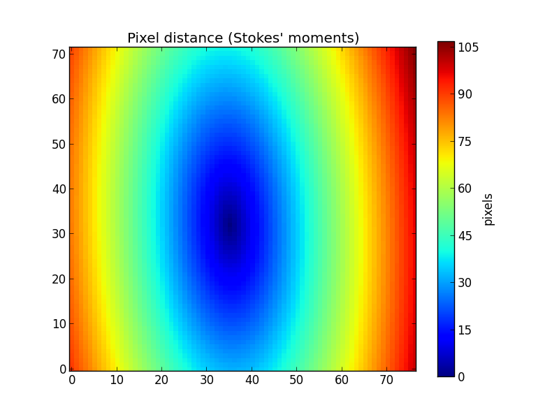
Now the distances match the geometry of the galaxy.

Galaxy scales

We also need to take into account that galaxies exist in all sizes and distances. This means that using pixels as a distance scale is not satisfactory. We need to convert it to a “natural scale” to compare the radial profiles of distinct galaxies.

We define the Half Light Radius (HLR_pix) as the semimajor axis of the ellipse centered at the galaxy center containing half of the flux in a certain band. In PyCASSO, we use qSignal, which is the flux in the normalization window.

The HLR is updated whenever setGeometry() is called. One can explicitly set the HLR using the HLR_pix parameter, or let it be determined automatically. Note that the HLR depends heavily on the ellipse parameters.

• Circular

>>> K.setGeometry(pa=0.0, ba=1.0)
>>> K.HLR_pix
9.334798311419563

• Ellipse

>>> pa, ba = K.getEllipseParams()
>>> K.setGeometry(pa, ba)
>>> K.HLR_pix
12.878480006876336
>>> K.HLR_pix
12.878480006876336
>>> K.HLR_pc
2545.9657503507078

In the last line we show the HLR in parsecs (HLR_pc), which may be handy sometimes. It is based on HLR_pix and parsecPerPixel.

Alternatively, one can think in terms of other property as a half-scale. This is achieved using the method getHalfRadius(). One alternate scale commonly used is the mass. To calculate the Half Mass Radius (HMR) use the following:

>>> K.getHalfRadius(K.McorSD__yx)
7.612629351561292

The input for this method must be a 2-D image.

Note: This uses the same computation as the HLR.

Calculating the radial profile of a 2-D image

Now that we have a scale to measure things in radial distance, it is useful to have a radial profile of things. First, let’s assume we have a 2-D image we want to get the radial profile, for instance, at_flux__yx. The method radialProfile() receives a 2-D image of a given property, a set of radial bins, an optional radial scale (it uses HLR by default) and returns the average values of the pixels inside each bin.

>>> HMR = K.getHalfRadius(K.McorSD__yx)
>>> bins = np.arange(0, 3+0.1, 0.1)
>>> bin_center = (bins[1:] + bins[:-1]) / 2.0
>>> at_flux__HLR = K.radialProfile(K.at_flux__yx, bins)
>>> at_flux__HMR = K.radialProfile(K.at_flux__yx, bins, rad_scale=HMR)
>>> plt.plot(bin_center, at_flux__HLR, '-k', label='at_flux (HLR)')
>>> plt.plot(bin_center, at_flux__HMR, '--k', label='at_flux (HMR)')
>>> plt.ylabel(r'$\langle \log t \rangle$')
>>> plt.xlabel(r'$R_{50}$')
>>> plt.title('at_flux')
>>> plt.legend()

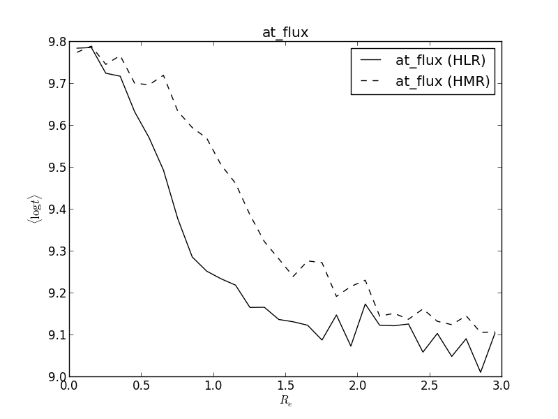
Now let’s explain the procedure. bins represent the bin boundaries in which we want to calculate the mean value of the property. It is not suitable for plotting, as it contains one extra value (len(bins) == len(at_flux__HLR) + 1). So, we calculate the central points of the bins, bin_center. Then, we proceed to calculate the radial profile of at_flux__yx, which is the average log. of the age, weighted by flux. We do so using HLR and HMR as a distance scale. The mass is usually more concentrated in the center of the galaxy, so that HMR < K.HLR_pix and therefore the plots look similar, but stretched. As with getHalfRadius(), the property used in the radial profile must be a 2-D image.

Calculating the radial profile of a N-D image

The method above only works for a 2-D image. Now, it would be nice to calculate the radial profile for higher dimensional data. For example, We have the surface distribution of mass in ages, McorSD__tyx, which is a 3-D array. One may be tempted to do a for loop, but there is a better tool for this job. The method radialProfileNd() works just like radialProfile(), except that you can use N-D arrays (and you can choose the reduce method, more on that later).

In this example, we want to plot a 2-D graph of the mass as a function of radius and age. We will use the Half Light Radius as a radial scale, so we don’t have to set the argument rad_scale as we did previously. We also don’t need the bin centers, as the plot method is fit for dealing with histogram data.

bin_r = np.arange(0, 2.5+0.1, 0.1) McorSD__tyx = K.McorSD__tZyx.sum(axis=1) logMcorSD__tr = np.log10(K.radialProfileNd(McorSD__tyx, bin_r, mode=’mean’)) vmin = -2 vmax = 4 plt.pcolormesh(bin_r, K.logAgeBaseBins, logMcorSD__tr, vmin=-2, vmax=4) plt.colorbar() plt.ylim(K.logAgeBaseBins.min(), K.logAgeBaseBins.max()) plt.ylabel(r’$log t$’) plt.xlabel(r’$R_{50}$’) plt.title(r’$log M_{cor} [M_odot / pc^2]$’)

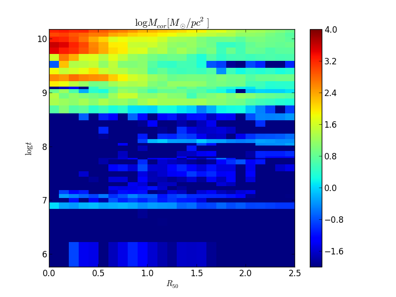
Note that to plot a pseudocolor mesh, one needs the mesh edges, so we have to use the radial bin edges (provided by bin_r), and the age bin edges. The property called logAgeBaseBins returns the age bin edges in log space, see it’s documentation for more details.

One can also compute the sum of the values (or the mean or median) inside a ring, using a pair of values as bins:

>>> Mcor_tot_ring = K.radialProfileNd(K.McorSD__yx, (0.5, 1.0), mode='sum') * K.parsecPerPixel**2

The multiplication by K.parsecPerPixel**2 is to convert from surface density to absolute mass. The mode keyword indicates what to do inside the bins. By default, the mean is computed. The valid values for mode are:

• 'mean'
• 'sum'
• 'median'

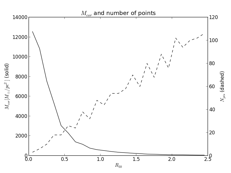
If the number of pixels inside each radial bin is needed, the keyword argument return_npts may be set. In this case, the return value changes to a tuple containing the radial binnned property and the number of points in each bin.

>>> bin_r = np.arange(0, 2.5+0.1, 0.1)
>>> bin_center = (bin_r[1:] + bin_r[:-1]) / 2.0
>>> McorSD__r, npts = K.radialProfileNd(K.McorSD__yx, bin_r, return_npts=True)
>>> fig = plt.figure()
>>> plt.title('$M_{cor}$ and number of points')
>>> ax1 = fig.add_subplot(111)
>>> ax1.plot(bin_center, McorSD__r, '-k')
>>> ax1.set_xlabel(r'$R_{50}$')
>>> ax1.set_ylabel(r'$M_{cor} [M_\odot / pc^2]$ (solid)')
>>> ax2 = ax1.twinx()
>>> ax2.plot(bin_center, npts, '--k')
>>> ax2.set_ylabel(r'$N_{pts}$ (dashed)')

Azimuthal and radial profile of a N-D image

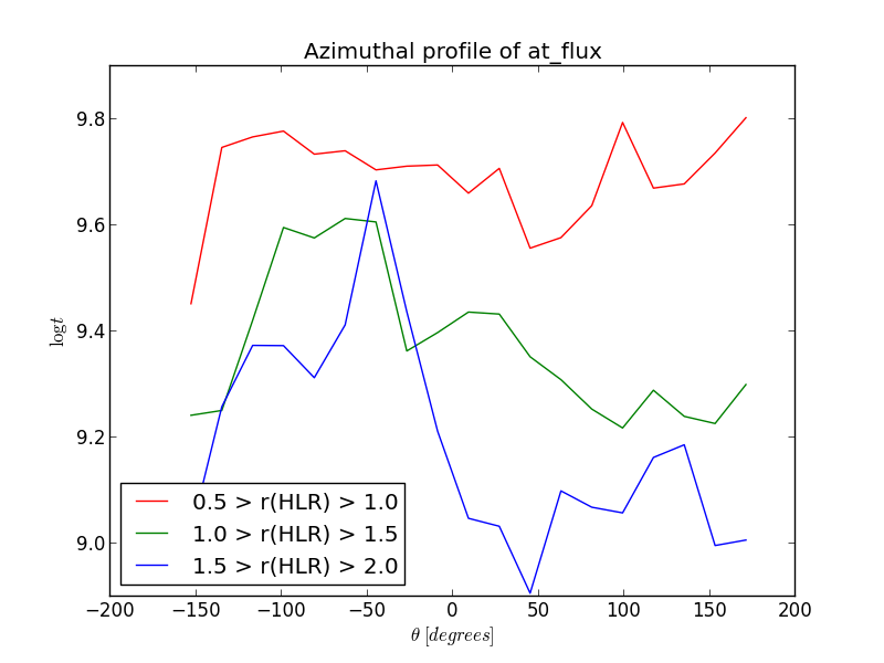
Still more generic than radialProfileNd() is azimuthalProfileNd(). It adds the capability of azimuthal profiles, based on the angles associated with each pixel. This angle is accessible using pixelAngle__yx, in radians. The method getPixelAngle() allows one to get the angle in degrees, or to get an arbitraty ellipse geometry, much like getPixelDistance().

In pycasso the pixel angle is defined as the counter-clockwise angle between the pixel and the semimajor axis, taking the ellipse distortion into account. Please look at getPixelAngle() for more details.

In the example below, we calculate the azimuthal profile of the log age, averaged in flux, inside three rings between 0.5, 1.0, 1.5 and 2.0 HLR.

>>> bin_a = np.linspace(-np.pi, np.pi, 21)
>>> bin_a_center_deg = (bin_a[1:] + bin_a[:-1]) / 2.0 * 180 / np.pi
>>> bin_r = np.array((0.5, 1.0, 1.5, 2.0))
>>> at_flux__ar = K.azimuthalProfileNd(K.at_flux__yx, bin_a, bin_r)
>>> plt.plot(bin_a_center_deg, at_flux__ar[:,0], '-r', label='0.5 > r(HLR) > 1.0')
>>> plt.plot(bin_a_center_deg, at_flux__ar[:,1], '-g', label='1.0 > r(HLR) > 1.5')
>>> plt.plot(bin_a_center_deg, at_flux__ar[:,2], '-b', label='1.5 > r(HLR) > 2.0')
>>> plt.title('Azimuthal profile of at_flux')
>>> plt.ylabel(r'$\log t$')
>>> plt.xlabel(r'$\theta\ [degrees]$')
>>> plt.legend()

Filling missing data

Coming soon.

Working with spectra

Coming soon.