Legacy API
Loading from FITS files
The process of loading data for a galaxy in a FITS file is similar to the HDF5 one. The main difference is that you only have to specify the path to the file. One should use sensible file names in this case. Using the same example, let’s load the data from the file 'K0001_synthesis_eBR_v20_q036.d13c512.ps03.k2.mC.CCM.Bgsd61.fits'.
>>> from pycasso.fitsdatacube import fitsQ3DataCube
>>> K = fitsQ3DataCube('K0001_synthesis_eBR_v20_q036.d13c512.ps03.k2.mC.CCM.Bgsd61.fits')
The object K is a fitsQ3DataCube, whick quacks almost exactly like a h5Q3DataCube, except for the dynamic loading of data present in the HDF5 implementation. Your script should work just like before.
Using very old scripts
There were several prototype versions of PyCASSO containing features which were abandoned, or renamed, or had changes in functionality. The class Q3DataCube is meant to be a backwards compatibility layer for older scripts that used these features.
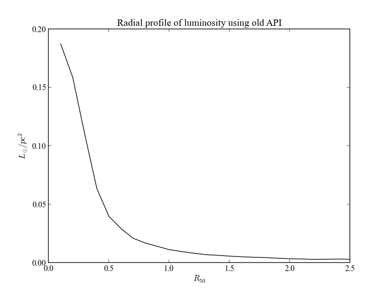
The main use for the old API is to convert from zone to XY notation, and produce radial profiles using the older dialect.
>>> from califa.Q3DataCube import Q3DataCube
>>> K = Q3DataCube('K0001_synthesis_eBR_v20_q036.d13c512.ps03.k2.mC.CCM.Bgsd61.fits')
>>> zyx = K.getZoneToYXTensor(extensive=True, dezonification=True)
>>> LobnSD__yx = np.tensordot(K.Lobn__z, zyx, (0, 0))
>>> ryx, bin_r, bin_area = K.getYXToRadialBinsTensor(d_r=0.1, \
rad_bin_ini=0.0, rad_bin_fin=2.5)
>>> LobnSD__r = np.tensordot(LobnSD__yx, ryx, [(0, 1), (1, 2)])
>>> plt.plot(bin_r, LobnSD__r, '-k')
>>> plt.xlim(0, 2.5)
>>> plt.xlabel(r'$R_{50}$')
>>> plt.ylabel(r'$L_\odot / pc^2$')
>>> plt.title('Radial profile of luminosity using old API')

All that could be easily attained using the methods zoneToYX() and radialProfile() without the hassle intermediary matrices and the order of the dimensions in tensordot.
Old API reference
- class califa.Q3DataCube.Q3DataCube(synthesisFile, circularProfile=True, runId=None, califaId=None, smoothDezonification=True)
- getZoneToYXTensor(extensive=True, dezonification=True)
Returns a tensor to transform from zone notation to spatial notation, with shape (zone, y, x). The normalization of the pixels can take into account the area of the zones or the luminosity weigth, using the following parameters:
Parameters : extensive : boolean
A.K.A. “normalize by zone area”. Use surface density when calculating the transformation from zone to spatial coordinates.
dezonification : boolean
Use image at 5650AA to weight pixels in the zones. This is used only when extensive=True.
Returns : zoneToYX : 3-D array
The transform tensor, shape (nZones, y, x).
Examples
To transform a cube named mycube, with axes (age, zone), into a cube with axes (age, y, x), one can perform the operation
>>> K = Q3DataCube(filename)
>>> zyx = K.getZoneToYXTensor()
>>> numpy.tensordot(mycube, zyx, (1, 0))
where 1 is the number of the zone axis in mycube, and 0 is the zone axis number in zyx.
- getYXToRadialBinsTensor(d_r, rad_bin_ini=0, rad_bin_fin=None, use_HLR_units=True, normalize_area=True)
Compute a tensor that transforms an array from zone binning notation to radial binning notation. Given the radial profile for this galaxy, this method calculates a tensor similar to the zonesToYXTensor, it transforms an image from spatial coordinates (x,y) to a radial profile.
Parameters : d_r : float
Radial step of the rings, in units of HLR.
rad_bin_ini : float, defaults to 0.0
Initial value for rad bins, in units of HLR.
rad_bin_fin : float, defaults to infinity
Final value for rad bins, in units of HLR.
use_HLR_units : boolean
If True, use the bins in HLR units. If False, use pixels.
normalize_area : boolean
If True, divide the tensor by the bin area.
Returns : YXToRad : array, shape (rad. bins, y, x).
The transform tensor.
bin_R : array of float
Radial bin outer edges.
bin_area : array of float
Radial bin area, in pixels.
See also
Examples
>>> c = Q3DataCube(file)
>>> yxToRad, bins, unused = c.getYXToRadialBinsTensor(d_r=0.2)
c.LobnSD__yx is the luminosity surface desity in each pixel. Compute the radial profile of the average luminosity surface density.
>>> radProf__R = np.tensordot(Lobn_tot__yx, yxToRad, [(0,1),(1,2)])
>>> plot(bins, radProf__R)
- getZoneToRadialBinsTensor(d_r, rad_bin_ini=0, rad_bin_fin=None, use_HLR_units=True, extensive=True, dezonification=False)
Return a tensor that transforms an array from zone binning notation to radial binning notation. Given the radial profile for this galaxy, this method calculates a tensor similar to the zonesToYXTensor, it transforms an image from spatial coordinates (x,y) to a radial profile.
Parameters : d_r : float
Radial step of the rings, in units of HLR_pix.
rad_bin_ini : float, defaults to 0.0
Initial value for rad bins, in units of HLR_pix.
rad_bin_fin : float, defaults to infinity
Final value for rad bins, in units of HLR_pix.
use_HLR_units : boolean
If True, use the bins in HLR units. If False, use pixels.
extensive : boolean
Use surface density when calculating the transformation from zone to spatial coordinates.
dezonification : boolean
Use image at 5650AA to weight pixels in the zones.
Returns : YXToRad : array, shape (y, x, zone)
The transform tensor.
bin_R : array of float
Radial bin outer edges.
bin_area : array of float
Radial bin area, in pixels.
See also
Examples
>>> c = Q3DataCube(file)
>>> zoneToRad, bins, unused = c.getZoneToRadialBinsTensor(d_r=0.2)
c.popx is luminosity fraction per zone. c.popx.shape is (ageBase, metBase, zone). Get the flux per unit area (?) for each zone.
>>> Lobn = c.popx / 100.0 * c.Lobs_norm
Total luminosity in each zone.
>>> Lobn_tot = Lobn.sum(axis=1).sum(axis=0)
>>> radProf = np.tensordot(Lobn_tot, zoneToRad, (1,1))
>>> plot(bins, radProf)
- findHLR_pix_CID()
TODO: Deprecated findHLR_pix_CID(). Find the half light radius using the image at 5650 Angstrom. Using radial bins of 1 pixel, calculate the cumulative sum of luminosity. The HLR is the radius where the cum. sum reaches 50% of its peak value.
Returns : HLR : float
The half light radius, in pixels.
See also
setGeometry
Notes
This value should be close to $dfrac{HLR_{circular}}{sqrt{b/a}}$.